1 Introduction
We’ve investigated how jobs are distributed across industry types and their focasted rate of change in different areas of Melbourne. Melbourne at the time of writing supports 527,738 jobs and an annual economic output of $215.213 billion according to remplan.
Key findings:
- Industries in finance, health and education are among the top ranking when it comes to future jobs
- Parkville and South Yarra suburbs is expected to have the most jobs in restaurants, entertainment, small jobs etc.
- Bigger financial firms and industries such as financial institutino, health and education happens closest to the CBD
From the data we have available the suburbs considered are Carlton, Parkville, Kensington and Sout Yarra. They are all scattered around the Melbourne central business district (CBD).
Show the code
# Create a map centered on Melbourne
melbourne_map = folium.Map(location=[-37.8136, 144.9631], zoom_start=13)

# Add a marker for Melbourne
# folium.Marker([-37.8136, 144.9631], popup='Melbourne').add_to(melbourne_map)

# Melbourne CBD coordinates
cbd_latitude = -37.8136
cbd_longitude = 144.9631

# Locations and their coordinates
locations = [
    ("Parkville", -37.778790, 144.942517),
    ("Kensington", -37.794152, 144.927635),
    ("Carlton", -37.800744, 144.966970),
    ("Docklands", -37.818903, 144.947014),
    ("South Bank", -37.823791, 144.962586),
    ("Port Melbourne", -37.836744, 144.928359),
    ("South Yarra", -37.839483, 144.995654),
    ("Torah", -37.841697, 145.013976)
]

# Create a map centered around Melbourne CBD
m = folium.Map(location=[cbd_latitude, cbd_longitude], zoom_start=14)

# Add markers for each location
for location in locations:
    name, latitude, longitude = location
    folium.Marker(location=[latitude, longitude], popup=name).add_to(melbourne_map)
melbourne_map
#melbourne_map.save("melbourne_map.html")
Make this Notebook Trusted to load map: File -> Trust Notebook
2 Jobs and employments
In the coming years the city of Melbourne is expected to see a steady and substantial increase in the jobs available across different industries.
We can quickly inspect what areas and industries have the most positive growth overall from the aggregated mean.
Show the code
grouped = jobs_industry.filter(pl.col('Industry Space Use') != 'Total jobs').groupby(['Geography', 'Industry Space Use'], maintain_order=True).agg([pl.col('Value').mean()]).sort('Value', descending=True).limit(8)
i_show(grouped)| Geography | Industry Space Use | Value |
|---|---|---|
| Loading... (need help?) |
Historically based on data from 2016 and 2021, the employment space of (Professional, Scientific and Technical Services) and (Financial and Insurance Services) has had the largest job capacity.
Show the code
# src: https://app.remplan.com.au/melbourne-lga/economy/trends/jobs?state=GLZrFN!az4VClkNKSYeGD6Uvqea6f0c4I6ZouPIWIKJhGI8hxx7AUwzL
jobs_historic = pl.read_csv('../data/melbourne-jobs-historically.csv', separator=';')
q = jobs_historic.sort('2021', descending=False)
q.filter(pl.col('Options').is_in(['Professional, Scientific and Technical Services',
                         'Financial and Insurance Services',
                         'Education and Training',
                         'Health Care and Social Assistance',
                         'Accommodation and Food Services']))

fig = go.Figure()
fig.add_trace(go.Bar(
    y=q['Options'],
    x=q['2021'],
    error_x=dict(type='data', array=q['2021'] - q['2016']),
    orientation='h'
))

fig.update_layout(
    title='Employments back in 2016 and 2021',
    xaxis_title='Employments',
    yaxis_title=None,
    yaxis=dict(autorange='reversed')
)

fig.show()
Overall Melbourne is considered a modern society that has the resources and ability to priotise education and economical growth. This is also reflected in the Gross Regional Product for the region which historically have also experiences a continous growth.
This is reinforced in the forecast. And especially so for the CBD. If we aggrate the job forecasts in area groups we see the following rates of change.
Show the code
jobs = pl.read_csv('../data/jobs_forecast.csv', ignore_errors=True, try_parse_dates=True)
jobs.columns
jobs.shape
jobs.describe()

jobs['Category'].unique()
list(jobs['Industry Space Use'].unique())

jobs_industry = jobs.filter(pl.col('Category') == 'Jobs by industry')

q = (jobs_industry
     .filter(pl.col('Industry Space Use') == 'Total jobs')
     .sort('Year')
     .groupby(['Geography', 'Year'], maintain_order=True)
     .agg(pl.sum('Value'))
     .with_columns([
         pl.col('Value').log().alias('Value_log'),
         pl.col('Year').cast(pl.UInt32)
     ]))
set(q['Geography'].unique())
q = q.filter(pl.col('Geography').is_in(['Melbourne (CBD)', 'Carlton', 'Kensington', 'Parkville', 'South Yarra', 'Southbank']))

sns.relplot(q, x='Year', y='Value', hue="Geography", kind="line")
plt.title("Job forecasts for areas")
plt.ylabel('Jobs')
plt.xlabel('Year')
plt.show()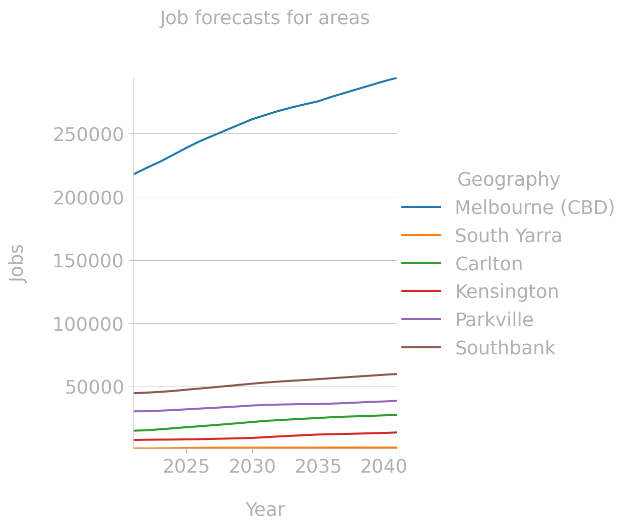
With Southbank and Parkville in close proximity to CBD being in the lead in regards to total jobs.
Next we can rank the different areas with respect to health, finance and education respectively starting with a bounded forecast up until 2025.
Show the code
jobs = pl.read_csv('../data/jobs_forecast.csv', ignore_errors=True, try_parse_dates=True)

jobs_industry = jobs.filter(pl.col('Category') == 'Jobs by industry')
q = jobs_industry.filter(pl.col('Geography').is_in(['Melbourne (CBD)', 'Carlton', 'Kensington', 'Parkville', 'South Yarra', 'Southbank']))

finance_ranks = q.filter(pl.col('Industry Space Use') == 'Finance and insurance').filter(pl.col('Year') <= 2025).with_columns(pl.col('Value').rank().alias('Rank')).sort('Rank', descending=True).filter(pl.col('Year') == 2025).limit(5)
finance_ranks[['Geography', 'Year', 'Rank']].limit(5)

healthcare_ranks = q.filter(pl.col('Industry Space Use') == 'Health care and social assistance').filter(pl.col('Year') <= 2025).with_columns(pl.col('Value').rank().alias('Rank')).sort('Rank', descending=True).filter(pl.col('Year') == 2025).limit(5)
healthcare_ranks[['Geography', 'Year', 'Rank']].limit(5)

education_ranks = q.filter(pl.col('Industry Space Use') == 'Education and training').filter(pl.col('Year') <= 2025).with_columns(pl.col('Value').rank().alias('Rank')).sort('Rank', descending=True).filter(pl.col('Year') == 2025).limit(5)

# Create ColumnDataSource for each data frame
finance_source = ColumnDataSource(finance_ranks[['Geography', 'Year', 'Rank']].to_pandas())
healthcare_source = ColumnDataSource(healthcare_ranks[['Geography', 'Year', 'Rank']].to_pandas())
education_source = ColumnDataSource(education_ranks[['Geography', 'Year', 'Rank']].to_pandas())

# Create DataTables for each data frame
finance_table = DataTable(
    source=finance_source,
    columns=[TableColumn(field='Geography', title='Geography'),
             TableColumn(field='Year', title='Year'),
             TableColumn(field='Rank', title='Rank')],
    width=400, height=200,
    index_position=-1  # Hide index column
)

healthcare_table = DataTable(
    source=healthcare_source,
    columns=[TableColumn(field='Geography', title='Geography'),
             TableColumn(field='Year', title='Year'),
             TableColumn(field='Rank', title='Rank')],
    width=400, height=200,
    index_position=-1  # Hide index column
)

education_table = DataTable(
    source=education_source,
    columns=[TableColumn(field='Geography', title='Geography'),
             TableColumn(field='Year', title='Year'),
             TableColumn(field='Rank', title='Rank')],
    width=400, height=200,
    index_position=-1  # Hide index column
)

# Create panels for each table
finance_panel = TabPanel(child=finance_table, title='Finance')
healthcare_panel = TabPanel(child=healthcare_table, title='Healthcare')
education_panel = TabPanel(child=education_table, title='Education')

# Create tabs layout
tabs = Tabs(tabs=[finance_panel, healthcare_panel, education_panel])
b_show(tabs)
The job forecast shows that the suburbs of South Yarra and Parkville have little traction for the before mentioned industries as they mainly consist of businesses such as restaurants and cafés. South Yarra has a history of being and attractive to live in with good proximity to CBD, schools, transportations and open lush parks and spaces.
It is also located right next to Toorak which is famous for its luxury residence and entreprenurs living there.
Next we will how they stand with a looser bound towards 2035, a change in 10 years.
Show the code
jobs = pl.read_csv('../data/jobs_forecast.csv', ignore_errors=True, try_parse_dates=True)

jobs_industry = jobs.filter(pl.col('Category') == 'Jobs by industry')
q = jobs_industry.filter(pl.col('Geography').is_in(['Melbourne (CBD)', 'Carlton', 'Kensington', 'Parkville', 'South Yarra', 'Southbank']))

finance_ranks = q.filter(pl.col('Industry Space Use') == 'Finance and insurance').filter(pl.col('Year') <= 2035).with_columns(pl.col('Value').rank().alias('Rank')).sort('Rank', descending=True).filter(pl.col('Year') == 2035).limit(5)
finance_ranks[['Geography', 'Year', 'Rank']].limit(5)

healthcare_ranks = q.filter(pl.col('Industry Space Use') == 'Health care and social assistance').filter(pl.col('Year') <= 2035).with_columns(pl.col('Value').rank().alias('Rank')).sort('Rank', descending=True).filter(pl.col('Year') == 2035).limit(5)
healthcare_ranks[['Geography', 'Year', 'Rank']].limit(5)

education_ranks = q.filter(pl.col('Industry Space Use') == 'Education and training').filter(pl.col('Year') <= 2035).with_columns(pl.col('Value').rank().alias('Rank')).sort('Rank', descending=True).filter(pl.col('Year') == 2035).limit(5)

# Create ColumnDataSource for each data frame
finance_source = ColumnDataSource(finance_ranks[['Geography', 'Year', 'Rank']].to_pandas())
healthcare_source = ColumnDataSource(healthcare_ranks[['Geography', 'Year', 'Rank']].to_pandas())
education_source = ColumnDataSource(education_ranks[['Geography', 'Year', 'Rank']].to_pandas())

# Create DataTables for each data frame
finance_table = DataTable(
    source=finance_source,
    columns=[TableColumn(field='Geography', title='Geography'),
             TableColumn(field='Year', title='Year'),
             TableColumn(field='Rank', title='Rank')],
    width=400, height=200,
    index_position=-1  # Hide index column
)

healthcare_table = DataTable(
    source=healthcare_source,
    columns=[TableColumn(field='Geography', title='Geography'),
             TableColumn(field='Year', title='Year'),
             TableColumn(field='Rank', title='Rank')],
    width=400, height=200,
    index_position=-1  # Hide index column
)

education_table = DataTable(
    source=education_source,
    columns=[TableColumn(field='Geography', title='Geography'),
             TableColumn(field='Year', title='Year'),
             TableColumn(field='Rank', title='Rank')],
    width=400, height=200,
    index_position=-1  # Hide index column
)

# Create panels for each table
finance_panel = TabPanel(child=finance_table, title='Finance')
healthcare_panel = TabPanel(child=healthcare_table, title='Healthcare')
education_panel = TabPanel(child=education_table, title='Education')

# Create tabs layout
tabs = Tabs(tabs=[finance_panel, healthcare_panel, education_panel])
b_show(tabs)
As we can see the CBD of Melbourne is flourishing with more jobs in finance and insurance.
Parkville houses one of Australia’s top hospitals both in its specializations but also as a teaching hospital. And since the general trend seems to favour more education this has a postive net effect on jobs om the parkville suburb.
2.1 Employment impact for the younger workforce
With the expected increase in population, especially for young adults. One might think that’s partly a result of an increase in job opportunities. Here we consider the younger group of women and the industry space of finance and insurance.
Show the code
jobs = pl.read_csv('../data/jobs_forecast.csv', ignore_errors=True, try_parse_dates=True)
jobs_industry = jobs.filter(pl.col('Category') == 'Jobs by industry').sort('Year')
jobs_industry = jobs_industry.filter(pl.col('Geography') == 'City of Melbourne')
jobs_industry = jobs_industry.filter(pl.col('Industry Space Use') == 'Finance and insurance')
#jobs_industry['Year'].max()

population = pl.read_csv('../data/population_forecast.csv', ignore_errors=True, try_parse_dates=True)
population = population.filter(pl.col('Geography') == 'City of Melbourne')
population = population.filter(pl.col('Gender') == 'Female')
# population = population.filter(pl.col('Age') == 'Average age')
population = population.filter(pl.col('Age') == 'Age 20-24')

joined = jobs_industry.join(population, on='Year', suffix='_population')
joined = joined.rename({"Value": "Jobs", "Value_population": "Population"})

corr = joined[['Year', 'Jobs', 'Population']]

f, ax = plt.subplots(figsize=(8, 5))

sns.heatmap(corr[['Year', 'Jobs', 'Population']].corr(), annot=True)

plt.title('Correlation matrix', size=12)
ax.set_xticklabels(list(corr[['Year', 'Jobs', 'Population']].columns), size=12, rotation=90)
ax.set_yticklabels(list(corr[['Year', 'Jobs', 'Population']].columns), size=12, rotation=0)
plt.show()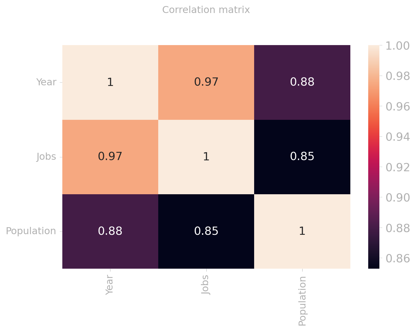
The last couple of years have seen an increase in automation and so called “smart banks”, also known as “fintech” institutions. They are keen on adopting the newest in technology and often houses employees with higher levels of education needed to sustain the digital demands. The positive correlation here is vague to assume alone on the population and jobs. But we still think it is fair to say that young adults recently graduated is attracted by these cooporate firms.
Reuse
CC