Show the code

import folium
import numpy as np
import pandas as pd
import polars as pl
import pandas as pd
import matplotlib.pyplot as plt
import matplotlib.image as mpimg
from bokeh.models import ColumnDataSource, FactorRange
from bokeh.io import output_notebook
from bokeh.models import ColumnDataSource
from bokeh.plotting import figure, show
from bokeh.sampledata.commits import data
from bokeh.transform import jitter
from bokeh.palettes import HighContrast3
from bokeh.plotting import figure, show
from bokeh.io import show
from bokeh.layouts import row, column
from bokeh.models import CustomJS, RadioButtonGroup
from bokeh.models import TabPanel, Tabs
from bokeh.plotting import figure, show
from bokeh.models import Paragraph
from bokeh.transform import dodge
from folium.plugins import HeatMap
from bokeh.palettes import Category20

output_notebook()

Loading BokehJS ...

1 Introduction

San Francisco is a renowned metropolis, situated in North California, USA, and serves as the commercial, financial, and cultural center of the region. This has attracted a significant influx of migrants to the city, and as of 2021, it has a population of 815,201 residents up to 2021, who have made a notable contribution to the city’s economy.

However, the city’s diverse socioeconomic challenges have also contributed to a high crime rate.

1.1 Dataset

In this story, we will examine the San Francisco Police Department’s (SFPD) Incient Report Dataset, which covers the period from January 2003 to May 2018.

The dataset contains information on criminal incidents reported in San Francisco, including the incident date, time, category, police district, latitude, longitude, and more. It comprises over 2 million records of crimes, with 35 columns of data.

The dataset reveals that 37 categories of crimes were recorded across the city of San Francisco.

1.2 Abstract

The aim of this report is utilizing the techniques of data visualization for the analytics of crime occured in San Francisco. The primary idea of this data analysis study is to obtain the insights from the observation, in order to evaluate the criminal situation for the past decades in San Francisco, as well as help prevent potential crimes in the future.

The data analysis will be based on Time-Series, Geographic and Interative Visualization respectively.

According to SFNext Index, with the exception of robberies, violent crime in San Francisco is below average for large cities. In 2019 and 2020, San Francisco ranked in the bottom half among major U.S. cities, with rates of 670 and 540 violent crime incidents per 100,000 residents, respectively. Hence, we are interested in how Robbery had increased the violent crime level in San Francisco.

2 Data Anlysis: Robberies in San Francisco

From January 2003 to December 2012, there were 35817 incidents of robbery in San Francisco reported to the police, while there were 32786 incidents of robbery reported from 2013 to 2022 (Data source).

As an overview, the robbery rate has decreased by 8.5% since the decade of 2003 to the last decade, however the number is not indicating a significantly decrease, which reflects the robbery is still a key factor that affect the level of crimes in San Francisco.

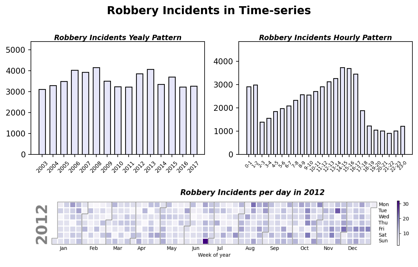
2.1 Timeseries: How the occurrence of Robbery changed over the time?

If we divide the time of the incidents into hourly timeslots, it becomes apparent that the number of robberies reaches its highest point between 2 and 3 pm and remains consistently high until 5 pm. After 5 pm, there is a sharp decline during the evening, but a secondary peak occurs between 1 and 2 am.Between 2 am and 2 pm, the number of incidents increases steadily.

Show the code

df_before_2018 = pl.read_csv('data/before_2018.csv').to_pandas()

focuscrimes = ['ROBBERY']

hour_of_day = [i for i in range(0,24)]
hourly_slots = {}
for i in range(len(hour_of_day)):
    if i+1 == len(hour_of_day):
        start = hour_of_day[i]
        end = hour_of_day[0]
        hourly_slots[start] = str(start) + "-" + str(end)
    else:
        start = hour_of_day[i]
        end = hour_of_day[i+1]
        hourly_slots[start] = str(start) + "-" + str(end)

df_before_2018["time_period"] = [hourly_slots[int(str(i).split(":")[0])] for i in list(df_before_2018['Hour'])]

yearly_pattern = df_before_2018.groupby(by=["Year", "Category"]).size().reset_index(name="Count")

yearly_pattern = yearly_pattern.loc[yearly_pattern['Category'].isin(focuscrimes)].reset_index(drop=True)

hourly_pattern = df_before_2018.groupby(by=["time_period", "Category"]).size().reset_index(name="Count")

hourly_pattern = hourly_pattern.loc[hourly_pattern['Category'].isin(focuscrimes)].reset_index(drop=True)


plt.figure(figsize=(7.5,5))
plt.suptitle("Robbery Incidents in Time-series" ,fontsize=14, y=1.0, fontweight='bold', color='black')

# Yealy trend
temp1 = yearly_pattern.loc[yearly_pattern['Category'] == 'ROBBERY'].reset_index(drop=True)
x = temp1["Year"]
y = temp1["Count"]
plt.subplot(2,2,1)
plt.title('Robbery Incidents Yealy Pattern', pad=-14, fontsize = 9, fontweight='bold', fontstyle="italic")
plt.bar(x, y, width=0.6, edgecolor="black", color='lavender')
plt.xticks(x, yearly_pattern['Year'].unique().tolist(), rotation=45, fontsize = 7)
plt.tight_layout()
plt.ylim(top=(np.max(y)+(np.max(y)*0.3)))

# Hourly trend
temp2 = hourly_pattern.loc[hourly_pattern['Category'] == 'ROBBERY'].reset_index(drop=True)
x = temp2["time_period"]
y = temp2["Count"]
plt.subplot(2,2,2)
plt.title('Robbery Incidents Hourly Pattern', pad=-14, fontsize = 9, fontweight='bold', fontstyle="italic")
plt.bar(x, y, width=0.6, edgecolor="black", color='lavender')
plt.xticks(x, hourly_slots.values(), rotation=45, fontsize = 6)
plt.tight_layout()
plt.ylim(top=(np.max(y)+(np.max(y)*0.3)))

# Calplot
img = mpimg.imread('Calplot_2012.png')
plt.subplot(2,1,2)
plt.imshow(img)
plt.axis('off')

plt.tight_layout()

From 2003 to 2017, we can see the incidents fluctuated accross years. Specifically, in 2010 and 2011, it has a significant decreased from 2008 and 2009. The Rand Corporation studied this phenomenon on a national level in 2010, concluding that the crime prevention benefit of hiring more officers is well worth the cost. Reference

However, there was a resurgence in incidents in 2012, with a noticeable gap from the previous year. After analyzing the robbery incidents data in 2012, we observed a marked increase in robberies on the final Sunday in June in San Francisco.

Further investigation revealed that this date coincided with the San Francisco LGBT Pride Parade, which started at Beale Street and Market Street and continued down to 8th Street.

2.2 Map: Where does robbery most likely take place?

Let’s examine the robbery locations on June 24, 2012, during the Pride Parade in San Francisco which typically occurs on Market Street(Reference: Wikipedia).

In the visualization of the robbery incidents data on the day when the Pride Parade occured, the three location marks Market Street, 8th Street and Beala Street respectively. The red dots indicates the location of the robberies taking place. It shows an obvious fact that in the 33 incidents recorded on 24 June 2012, most of the crimes happened in the range of the routes that the parade covered.

Show the code

df_before_2018 = pl.read_csv('data/before_2018.csv').to_pandas()

df_robbery = df_before_2018.loc[df_before_2018['Category']=="ROBBERY"]
df_robbery = df_robbery[df_robbery["Year"] == 2012]
df_robbery_pride = df_robbery[df_robbery['Date'] == '2012-6-24']

SF_map = folium.plugins.DualMap(location=[37.77919, -122.41914],
                    zoom_start = 12,
                    tiles = "openstreetmap")

constraint = (df_before_2018['Category'] == 'ROBBERY') & (df_before_2018['Year'] >= 2011) & (df_before_2018['Year'] <= 2012) & (df_before_2018['Resolution'] == "ARREST, BOOKED")
df_robbery_heat = df_before_2018.loc[constraint].reset_index(drop=True)


get_XY = list(zip(list(df_robbery_pride["Y"]), list(df_robbery_pride["X"])))

SF_map = folium.Map([37.77919, -122.41914], zoom_start=13, tiles = "openstreetmap")
folium.Marker([37.77351584799628, -122.42148577465927], popup="Market Street").add_to(SF_map)
folium.Marker([37.78907067508782, -122.3929690574588], popup="Beala Street").add_to(SF_map)
folium.Marker([37.77295458293956, -122.40701151351163], popup='8th Street').add_to(SF_map)

for x,y in get_XY:
    folium.CircleMarker([x, y],
                    radius=2,
                    color='red',
                    ).add_to(SF_map)


x_y_robbery = list(zip(list(df_robbery_heat["Y"]), list(df_robbery_heat["X"])))

HeatMap(x_y_robbery, min_opacity=0.35, overlay=True).add_to(SF_map)

SF_map

Make this Notebook Trusted to load map: File -> Trust Notebook

The incidence of robbery is relatively high in the near Market Street, indicating that criminals are more prone to commit robbery in crowded areas, thus increasing their chances of escape. Additionally, the buildings and blocks in the Market Street area are more densely packed, offering additional cover and refuge for criminals.

This observation also aligns with the result of the heatmap regarding robbery occurrence in 2011 and 2012, as the map above indicates. It reveals the fact that areas with a high concentration of stores and a large population, along with a complex urban infrastructure, are more susceptible to robbery incidents.

However, despite the fact that the Tenderloin district where Market Street located had the highest number of robbery incidents, the data implies that it was not the most active police district. This fact can be counted to the assumption that there was a lack of police power resources in Tenderloin district.

2.3 Interactive Visualization: Police district performance

How does the police perform in the different districts?

As the activities of police can be a key factor that effect on the crime rates, we therefore would like to see how the number of crimes has changed based on different districts. The data are used and maintained by the Police Department, which indicates that the number of records reflects the activities of the police districts. The incidents that are not reported and recorded is excluded to the scope of our discussion.

We normalized the occurrences of crime incidents and then created an interactive visualization to enable easy inspection of the normalized number of incidents in each police district.

Show the code

dataset = pl.read_csv('data/before_2018.csv')

data = (
  dataset
  .groupby(['Hour', 'PdDistrict'])
  .agg(pl.count().alias('Occurence'))
  # .with_columns(pl.col('count').alias('Occurence'))
  .sort('Hour')
).to_pandas()

data['Sum'] = data.groupby('PdDistrict')['Occurence'].transform('sum')
data['Norm'] = data['Occurence'] / data['Sum']
data = data.pivot_table(index='Hour', columns='PdDistrict', values='Norm').reset_index()

districts = set(['RICHMOND', 'TARAVAL', 'MISSION', 'INGLESIDE', 'SOUTHERN', 'NORTHERN', 'TENDERLOIN', 'CENTRAL', 'BAYVIEW', 'PARK'])

source = ColumnDataSource(data)
hours = data['Hour'].unique()
hours = sorted(hours)
p = figure(title="Police District", x_axis_label='Hour of the day', y_axis_label='Percentage Frequency', 
           x_range = FactorRange(factors=[str(hour) for hour in hours]))
bar = {}
for indx, i in enumerate(districts):
    bar[i] = p.vbar(x="Hour", top=i, width=0.3, 
                    source=source, legend_label=i, muted_alpha=0.2, muted=False, color=Category20[14][indx])
p.legend.title = "Police District"
p.legend.location = "top_left"
p.legend.click_policy = "mute"
p.legend.label_text_color = "black"
p.legend.title_text_color = "black"
show(p)

Through the interactive visualization, users are able to select the district they are interested in to observe the data. From the visualization, we can first get the information that each police district has the similar pattern of activities: almost all districts has the relatively high frequency of criminals during 7 am to 23 pm, with the peak at 11 am. It can be reflected that there are more active police resources working during day shift.

However the normalized occurrence of crimes has decreased by half during 0 am to 7 am, and the bottom occurs at the timeslot of 4 am to 5 am. In general, Park District, Taravel District and Southern District were likely to have the best performance due to the relatively larger amount of crime records. Police in Tenderloin District has better performance than Central District at the timeslots of 4-7 am and 12-16 pm, however, however it was less performed than Central District from 17 pm to 3 am.

However, by inspecting in the data of the total occurrence of all categories of crimes, we were not able to catch an apparent correlation between the pattern of crimes and the activity of police districts.

3 Conclusion

In summary, we conducted an analysis of robbery incidents in San Francisco from 2008 to 2012 using time series analysis.

Our investigation revealed that robbery incidents generally peak during the summer months, as indicated by the calendar plots spanning 2003 to 2017.

We also found that the busiest city center is more prone to crime. However, we did not observe a positive correlation between police activities in each district and the number of robbery incidents.

SF Crime Data Analysis and Visualization

1 Introduction

1.1 Dataset

1.2 Abstract

2 Data Anlysis: Robberies in San Francisco

2.1 Timeseries: How the occurrence of Robbery changed over the time?

2.2 Map: Where does robbery most likely take place?

2.3 Interactive Visualization: Police district performance

3 Conclusion

Reuse